


Microsoft Excel is one of the most popular spreadsheet software that enables companies to efficiently manage their data. It’s a data analysis tool which offers powerful and efficient analytics features empowering data analysts to make intelligent business decisions. In this article we are going to discuss the top 15 most powerful excel functions for data analysis.
But before we dive into using the formulas, it’s important to learn the difference between two related concepts when we talk about Excel, that is, data analysis and data analytics.
Data analysis and data analytics are two different but closely related concepts. The process of Data analysis encompasses three tasks, cleaning, transforming and analyzing the data. Data analytics, on the other hand, is a broad term and also includes data collection, organization, and data communication. Excel empowers companies to enable data analysis by offering powerful tools for cleaning, transforming and analyzing the data.
Preparing your Dataset
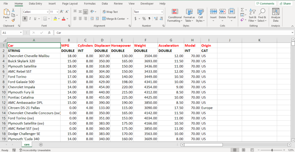
Take a look at the cars dataset we used in this tutorial. It’s available for free at Telecom Paris by James R. Eagan.
The dataset contains 408 rows, with 405 rows representing cars each carrying 8 columns representing its characteristics such as MPG, Acceleration, and Country of origin. All operations for this article are performed with reference to this data set.
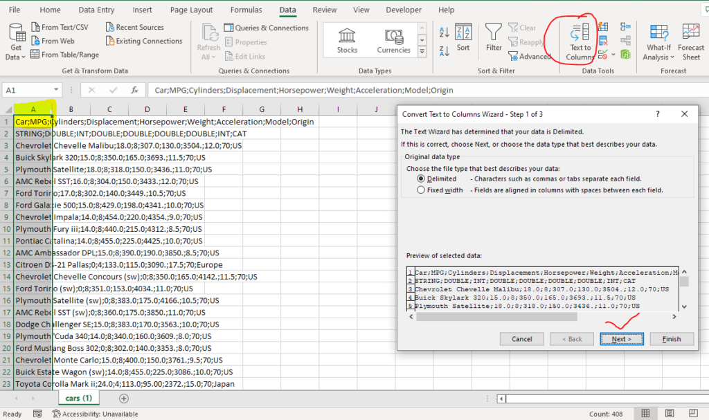
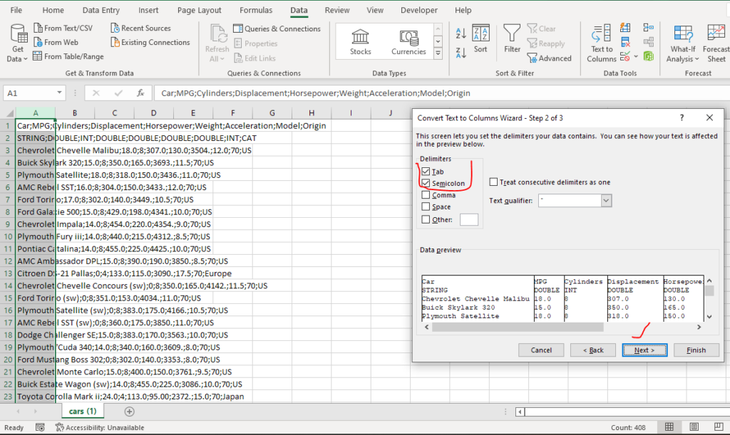
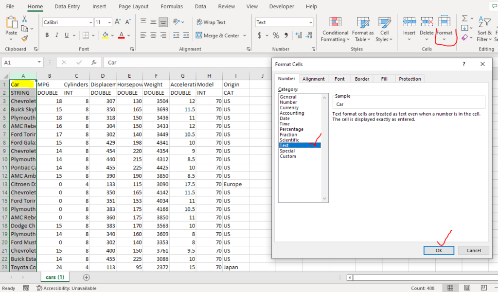
IMPORTANT: Before applying excel formulas, please make sure that your dataset is converted from ‘text to column’ from the ‘Data tab’, with delimiter ‘;’. The following snippets guide you through the process.
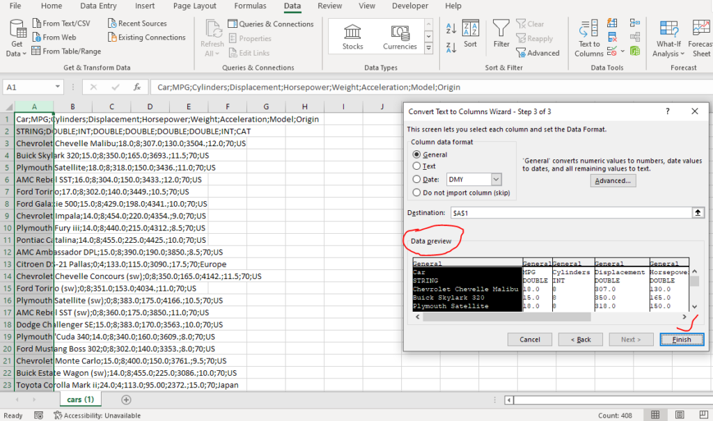
Also make sure you set data type for each column by using cell format tool in ‘Home tab’. Set the data types to Number or Text as required by the columns. If the data types are not set, Excel will assign general data types to all the columns and the functions stated below would not work on them.
List of Excel functions
Data analysts would want to explore data in limitless ways and therefore, in this article, we present various Excel functions that range from arithmetic operations to finding character length and looking up a value from within a column.
SUM()
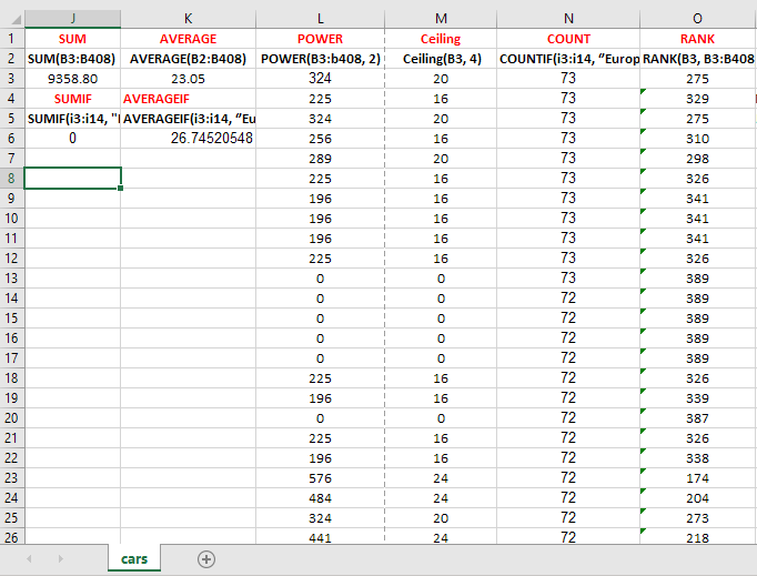
The SUM() function calculates the sum of cell values. It’s always applied on Numeric data types. Within the parentheses, specify a range as in =SUM(B3:B408) to apply addition operation on the set of values specified by the range.
AVERAGE()
The AVERAGE() function calculates the average of cell values. Just as the SUM(), it’s too always applied on Numeric data types. Within the parentheses, specify a range as in =AVERAGE(B3:B408) to apply average operation on the set of values specified by the range.
POWER()
This function takes the power of any input value. POWER(number, power) function takes two input parameters, number in the cell, and power value. You can also specify a cell range as in =POWER(b3:b408, 2) to apply a power of 2 over the cells B3, to B408. The POWER() function will spill the result in more than one row for multiple cells.
CEILING/FLOOR
These two functions round off any numeric value to either up or down the nearest multiple of a number of significance. Rounding to the nearest multiple means that the result will be the closest number that is the multiple of the specified significance value in either direction.
For example, =Ceiling(18, 4) will round off the number 18 up the nearest multiple of 4, which in this case is 20. While =Floor(18, 4) will round off the number 18 down the nearest multiple of 4 which in this case is 16.
For the case of applying formula over a range of cells in a column for any significance value ‘x’, CEILING(b2:b7, x) will return the result over the cells between b1, and b8. In this case the CEILING() function will spill the result in more than one row for multiple cells.
SUMIF()
It’s the SUM() functionality but it offers more flexibility by allowing you to sum over a specified criteria. It takes at least two parameters, one is the range to be summed up, and the other is criteria. For example, you want to sum the cell values b3 to b7, but you want to sum only those that are greater than 5. You would put something like this, =SUMIF(b3:b7, “>5”).
For the case where you want to sum values in a separate column and specify criteria from another column you would input three parameters. Take an example, you want to sum the cells b3:b14 but this time you want to sum only those cells in the B column that represent the country Europe in the I cell of the excel sheet. So you would put something like this: =SUMIF(i3:i14, ‘’Europe”, b3:b14). Note, in this case, the range to be summed is not at the start of the formula, rather it’s in the end.
AVERAGEIF()
Similar to SUMIF(), this function will output the average values over a criteria defined. You will input at least two parameters, the range to be averaged and the criteria for which the rage values fulfill. For example, to average the first five cell values in column B greater than 5, enter the following: =AVERAGEIF(b3:b7, “>5”).
For more enriched criteria, the formula takes three parameters. =AVERAGEIF(i3:i14, ‘’Europe”, b3:b14) will take average on cells b3 to b14 where the cell values in the I column are “Europe”. Note, in this case, the range to be averaged is not at the start of the formula, rather it’s in the end.
COUNTIF()
Now that you know what an if-embedded function would do for you, this function is pretty straight forward and might be the easiest to understand. It will count the number of cell values that fulfill a defined criteria.
For example, to count the first five cell values in column B that are greater than 5, enter the following: =COUNTIF(b3:b7, “>5”). The function =COUNTIF(i3:i408, ‘’Europe”) will only count cell values over i3 to i408 where the cell values in the I column are “Europe”.
RANK()
This function is immensely useful in data analysis and it ranks a numeric data value in ascending or descending order by comparing its value in the list of values. It takes three arguments, a data value that is to be ranked, a list of numeric values for comparison, and an order number. If order number is 0, it ranks in descending order, and if order number is 1 the function will rank the numeric value in descending order.
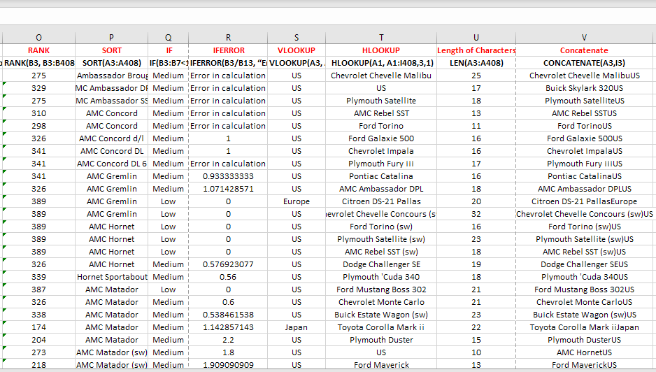
For example, =RANK(B3, B3:b408, 0) will rank value in b3 in descending order.
SORT()
While RANK() functions to determine the rank of a value as its place in the list, SORT() will simply output a sorted version of the data. Unlike RANK() it’s equally useful for both numeric and text data types. To sort values in ascending order, you would put function as: =SORT(A3:A408) while for descending order sort function, you would increase the input parameters and write something as: =SORT(A3:A408, 1, -1) where -1 denotes a sort operation in descending order.
IF()
IF() is one of the most popular functions in excel and it allows you to compare values and outputs a logical value or your mentioned result if the comparison is either True or False. It’s used for both numeric and text data types. For example, in our cars dataset we want to categorize cars based on how much mileage they cover per gallon (MPG). For this we write the following function in formula bar: =IF(B3:408<10,”Low”, “Medium”).
The above function will output Low if MPG is less than 10, and medium otherwise.
IFERROR()
IFERROR() offers an amazing functionality of handling errors in a formula.This means that it will return a result you specify when there’s error in the formula. An error shows that the result of calculation is false.
An error example could be in arithmetic operation when you divide a value by 0. In this case you would write something as: =IFERROR(B3/B13, “Error in calculation”), it will output Error in calculation. If the result is true, the calculated value is the output.
VLOOKUP()
We have seen arithmetic and count functions over a range based on criteria using SUMIF(), AVERAGEIF() and COUNTIF().
Now let’s take a look at how we can find values from a table based on a criteria. VLOOKUP() finds values in a column (or as we say by row).
To simplify the function, a VLOOKUP() would need following input parameters: =VLOOKUP(What you want to look up, where you want to look for it, the column number in the range containing the value to return, return an Approximate or Exact match – indicated as 1/TRUE, or 0/FALSE).
For example, in our dataset, we want to look for the origin of the car ‘Chevrolet Chevelle Malibu’. We would use VLOOKUP and write something like this: =VLOOKUP(A3, A3:I408,9,0). It will return the output of: US.
Please note that VLOOKUP will not work if the index of the column of the value you are looking for (the first parameter after open parenthesis) is greater than the column index mentioned in the third parameter.
HLOOKUP()
HLOOKUP() is used to find values in a row (or as we say by column). A column is specified from the top row of the table and a row index is provided to find the value in the same column.
For example, in our dataset, we want to look for the cars in a specific row. We would use HLOOKUP and write something like this: =HLOOKUP(A1, A1:I408,3,1). It will return the output of: Chevrolet Chevelle Malibu.
LEN()
LEN() calculates the number of characters in each cell. It takes a single input parameter that is the cell value for which character length is required.
CONCATENATE()
It’s an immensely useful function when combining different data into a single entity. This function embeds a number of data cells together. The syntax is =CONCATENATE(A3,I3).
Grow your skills as Business Analyst!
Excel is termed as one of the top skills for business analysts other than SQL and PowerBI. With little time spent on practicing these top 15 functions, you would become better at using Excel for data analysis. At this point, we would urge you to practice these top 15 functions at your side and explore other 500+ functions to further enhance your analytical skills.
We wish you happy learning!
Further to add to the article, although we have SO many other powerful tools available to draw forensics from data, the industries still prefer using excel considering that it has become user friendly and our eyes have become acquaintance to the layout.
That’s absolutely right! It’s a fact that Excel has become one of the most powerful tool in data analytics that’s commonly available to almost every person.