


SQL is by far the most widely accepted programming language across the data analytics industry. The 40 year old language is well documented and is very easy to learn.
In this article, we look at 6 advance SQL statements with examples that will help you to manipulate data in a more flexible and powerful way.
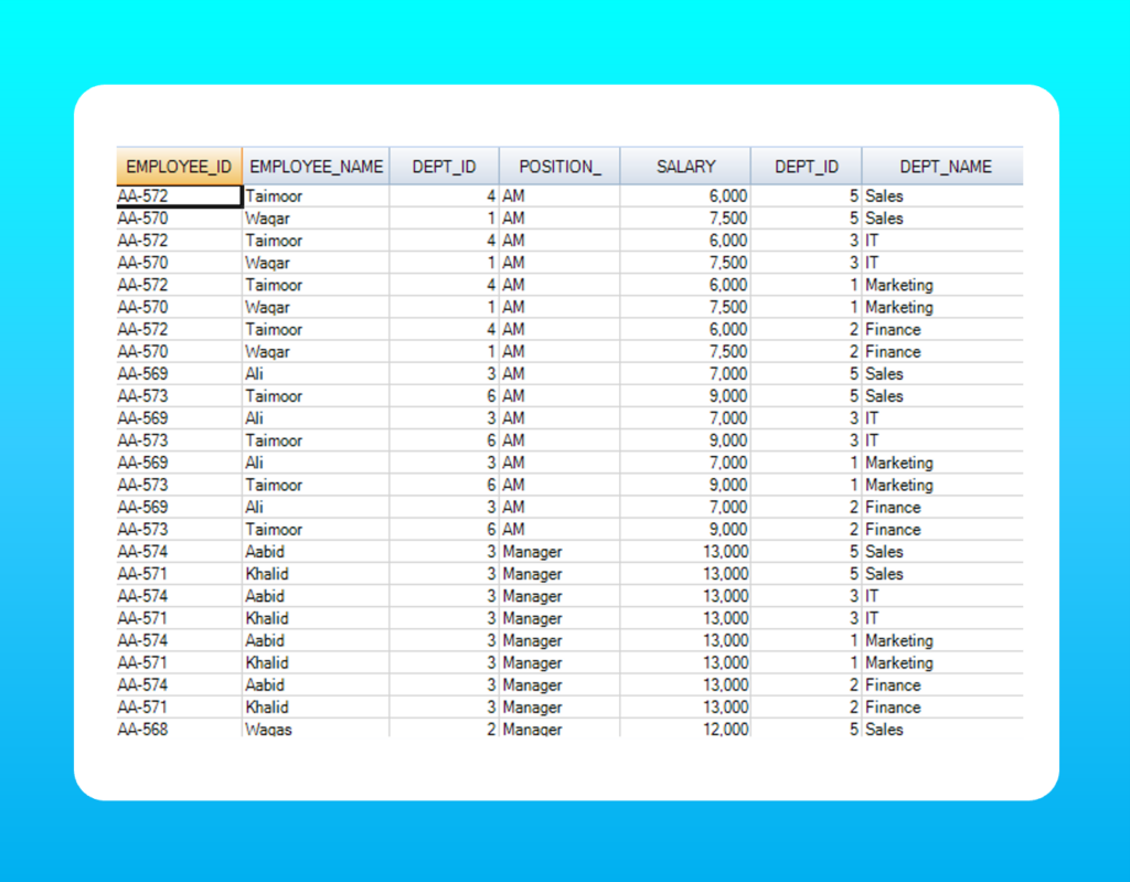
IMPORTANT: All examples provided in this article have been tested on our custom database ‘Dice’ that consists of two tables; ‘Employee’ and ‘Department’. These tables are shown as follows:
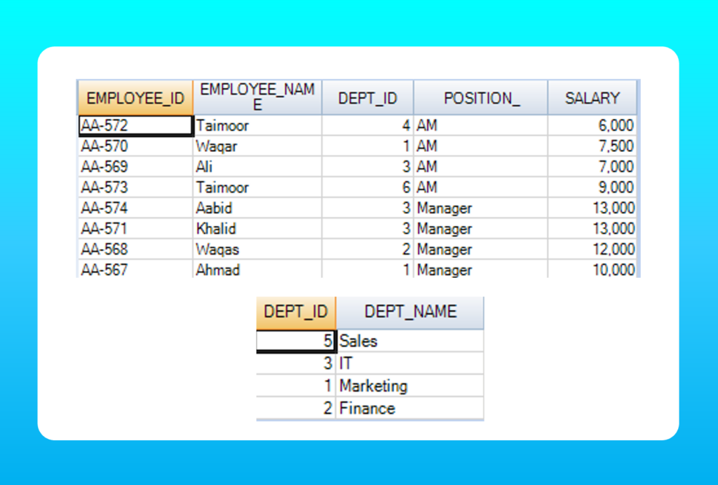
Now let’s see the SQL statements one by one.
Table of Contents
SQL JOIN
Oftentimes while manipulating data we want to combine information from two tables. This is done using SQL JOIN statements.
For two tables to join they must contain a common column.
Practical Tip: In the modeling stage of a database, a data modeler puts a unique column of one table (the primary key; pk) in the other table (a foreign key; fk) to enable join in the later stage of data engineering.
There are a number of ways we can achieve ‘join’ operation between tables.
INNER JOIN
Inner join is by far the most simple join and combines two tables while displaying only the rows that match as per the joining criteria.
All unmatched values are discarded in the inner join.
Inner join works by sequentially matching a row of one table with all rows of the other table as per the joining criteria.
Syntax: INNER JOIN column_name
ON table_1.pk = table_2.fk;
Where the ON clause represents the joining criteria (often referred to as the stitching criteria) and specifies those columns that are to be matched in both tables. Here the columns are pk (primary key) and fk (foreign key) residing in both tables respectively.
As an application of inner join, consider the following example.
We want to filter employees from the employee table whose departments demonstrated excellent performance. We have a department table that carries the highest performing department names.
We can use inner joins to filter out the employees from the employee table using the following query.
SELECT d.dept_name, e.employee_name, e.dept_id
FROM employee e
JOIN department d
ON e.dept_id = d.dept_id;
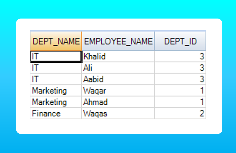
Here ‘dept_id’ is the primary key in ’employee’ and resides as foreign key in ‘department’.
Now, what if a data analyst wants to view the rest of the employees from other departments alongside as well?
SQL Left joins come in handy for this!
LEFT JOIN/RIGHT JOIN
A left join will output all rows of the first table (left table) but only matched values from the second table (as per the joining criteria).
In the resulting table you might see ‘null values’ that specify the unincluded values from the second table.
Syntax: LEFT JOIN column_name/ RIGHT JOIN column_name
ON table_1.pk = table_2.fk;
We use the following query to view both; employees from the highest performing department and the rest of the employees in the employee table.
SELECT *
FROM employee e
LEFT JOIN department d
ON e.dept_id = d.dept_id;
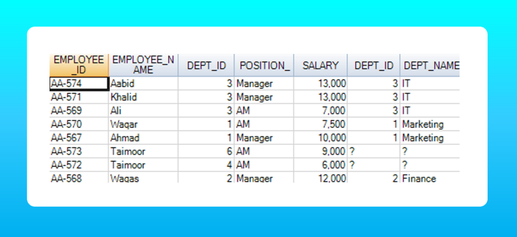
IMPORTANT: Total rows in left join = total matched rows + (unmatched rows from first table)
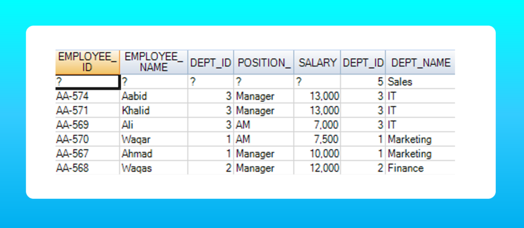
Similarly, a right join will keep all rows from the second table (right table) but will only keep matched values from the first table.
Total rows in right join = total matched rows + (unmatched rows from second table).
SELECT *
FROM employee e
RIGHT JOIN department d
ON e.dept_id = d.dept_id;
CROSS JOIN
Cross join is a ‘notorious’ operation. It takes a lot of computational power and memory to generate and store output. We avoid its use in practical scenarios.
A cross join simply combines each row of one table with all rows of the other table (similar to a ‘combination operation’ in mathematics). There’s no stitching criteria because we are simply making combinations between two tables.
The resulting table is a huge table that carries all possible combinations of data elements.
Syntax: CROSS JOIN column_name.
In our database, the employee table has a total of 8 rows and the dept table carries 4 rows. The cross join operation results in the number of rows = 8×4 =32.
SELECT *
FROM employee e
CROSS JOIN department d;
SQL Aggregate Functions
SQL aggregate functions perform mathematical operations on data.
There are five number of aggregate functions; COUNT(), SUM(), MAX(), MIN(), and AVG().
Syntax: SELECT aggregate function(column_name) FROM table_name
Aggregate functions are used within the SELECT statement.
It’s worth noting here, each aggregate function outputs a single value against the whole column. Due to this particular reason we can’t query a column when using an aggregate function.
As we would see later in the article, the window aggregate functions are more useful when querying columns alongside aggregate results.
SQL GROUP BY
It’s an immensely useful function that offers frequent support in the daily operations of a data analyst.
GROUP BY arranges identical data of a column into groups and is used in combination with SELECT clause and Aggregate functions.
Syntax: GROUP BY(column_name).
Use GROUP BY on a column to group similar data and then apply aggregate functions over another column to aggregate the data within each group.
For example, we want to view the average salary within each department.
SELECT position_, AVG(salary) FROM employee
GROUP BY(position_);
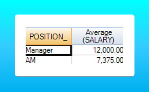
The position_ column is grouped and reduced to two rows, and for each group an average function is applied.
Practical tip: Use GROUP BY after WHERE clause but before ORDER BY or LIMIT.
Disadvantage: GROUP BY reduces the number of rows in the resulting table and therefore you cannot SELECT original columns of the table when you apply GROUP BY.
This drawback of GROUP BY leads us to the ‘window functions in SQL’; OVER().
SQL OVER()
A window aggregate function is defined as “the one which allows aggregate functions to output a result against each window (row) ”.
OVER() is a useful window function and commonly used with aggregate functions. It offers the flexibility to display the aggregated results against each row of the original table.
Syntax: SELECT aggregate function(column_name) OVER() FROM table_name
Note that OVER() is used within the SELECT clause.
Example:
SELECT employee_name, SUM(salary) OVER()
FROM employee;
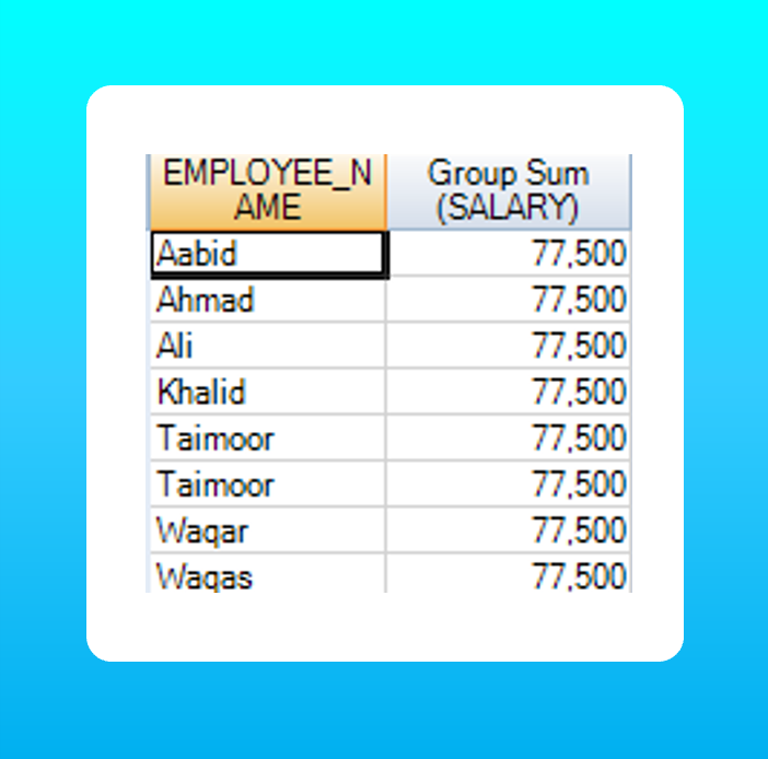
Note the result table contains the same rows as the original table.
SQL PARTITION BY
PARTITION BY is a sub clause of OVER() function and it’s immensely useful as you will witness shortly.
Syntax: SELECT aggregate function(column_name) OVER(PARTITION BY column_name) FROM table_name
OVER( PARTITION BY column_name) is like a GROUP BY column_name that groups similar data in a column. The difference lies in that now you can query multiple columns in the SELECT clause which was not earlier possible with GROUP BY.
The result table contains the same rows as the original table.
For example, I want to see how many employees are at Managers position and AM position. The following query will do it.
SELECT employee_name, position_, COUNT(employee_name) OVER(PARTITION BY position_)
FROM employee
WHERE dept_id IN (SELECT dept_id FROM department)
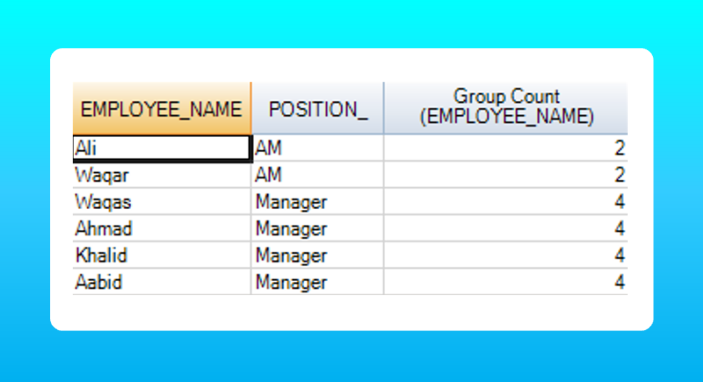
As you can see in the results table, there are a total of 2 employees at AM position while the total employees at the Manager position are 4. The result is displayed against each row.
SQL ORDER BY
ORDER BY is a powerful clause in SQL which can be applied to more than one column. It’s also used as a sub clause in the OVER() function.
Syntax: SELECT column_1, column_2, …
FROM table_name
ORDER BY column_1 ASC|DESC,… column_n ASC|DESC
ORDER BY column_1 ASC|DESC sorts the contents of column_1 in ascending order when ASC is specified, or descending order if DESC is specified.
If the order key is not mentioned, ASC is chosen by default.
ORDER BY Multiple column (Major sort and Minor sort)
If more than one column is specified in ORDER BY, then the first column uses major sort and gets sorted on priority while the second column uses minor sort and gets sorted after the major sort.
Note the order of the first column is maintained when the second column is sorted.
ORDER BY in OVER()
Order by is used as a sub clause in over() function. It serves as a sorting function with the benefits of flexibility in querying columns in the SELECT statement.
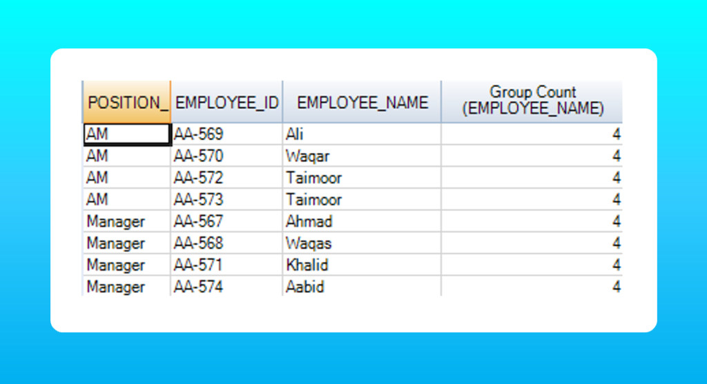
For example, I want to see how many employees are at Managers and AM positions against their sorted employee ID. The following statement will be used:
SELECT position_, employee_id, employee_name,
COUNT(employee_name) OVER(PARTITION BY position_ ORDER BY employee_id)
FROM employee;
Take a Free Course!
It’s a fact that almost all database service providers across the data analytics industry use SQL as their default programming language. To know more about it you can refer to SQL and Database management for an overview.
Stating that, it creates a high demand for SQL as a basic skill in data analytics job roles. There are some renowned platforms that offers free training on SQL for free; we suggest codecademy and coursera.
PS once you get hands on in SQL, Hackerank is another amazing platform that could test your SQL ability through interesting and challenging problems.